Working with synthetic observations
Transmission spectrum
An atmosphere’s transmission spectrum is the sum of absorption spectra of atoms and molecules present in the atmosphere.
The methodology of obtaining the information needed to calculate the synthetic transmission spectrum using the Met Office Unified Model (UM) output is reported in Lines et al. (2018):
https://academic.oup.com/mnras/article/481/1/194/5078378 (publisher)
https://arxiv.org/abs/1808.05887 (arXiv)
Please note that Lines et al. (2018) take into account the atmospheric conditions in the columns on the nightside of the planet limb only. The instructions on how to obtain the same information for the dayside are here:
http://exoclimatology.com/wiki/index.php?title=Transmission_Spectra (requires login)
aeolus.synthobs requires the following inputs to calculate the synthetic transmission spectrum:
spectral_file- SOCRATES spectral file used by the UMstellar_constant_at_1_auin [W m-2]stellar_radiusin [m]planet_top_of_atmospherein [m], which is the extent of the planetary atmosphere (usually, it is the sum of the planetary radius and the height of the model domain)planet_transmission_day- UM m01s01i755 output (for hot Jupiters) from the dayside calculationplanet_transmission_night- UM m01s01i755 output (for hot Jupiters) from the nightside calculation
Below is an example of such a calculation that uses a test spectral file and two test UM output files. The files are available at https://github.com/exoclim/aeolus_data.
Import relevant packages
[1]:
import warnings
from pathlib import Path

import iris
import iris.cube
import iris.quickplot as qplt
import matplotlib.pyplot as plt
import numpy as np
[2]:
from aeolus.model import um
from aeolus.synthobs import (
    calc_stellar_flux,
    calc_transmission_spectrum,
    calc_transmission_spectrum_day_night_average,
    read_normalized_stellar_flux,
    read_spectral_bands,
)
[3]:
warnings.filterwarnings("ignore", module="iris")
plt.rcParams["mathtext.default"] = "regular"
[4]:
iris.FUTURE.datum_support = True
[5]:
# Note that the file paths should be pathlib.Path-like objects, not just plain strings!
TEST_DIR = Path.cwd().parent / "tests" / "data" / "test_data"
Provide the required inputs
[6]:
spectral_file = TEST_DIR / "spectral" / "sp_sw_500ir_bd_hatp11"
data_file = TEST_DIR / "netcdf" / "planet_transmission_day.nc"
planet_transmission_day = iris.load_cube(data_file)

# To keep the units of stellar and planetary parameters, store the parameters as iris cubes
stellar_constant_at_1_au = iris.cube.Cube(
    300.85538168664425, units="W m-2", long_name="stellar_constant_at_1_au"
)
stellar_radius = iris.cube.Cube(475026500.0, units="m", long_name="stellar_radius")
planet_radius = iris.cube.Cube(27195379.0, units="m", long_name="planet_radius")
planet_domain_height = iris.cube.Cube(1.8e6, units="m", long_name="height_domain")
planet_top_of_atmosphere = planet_radius + planet_domain_height
Check if the information about the spectral bands is read in correctly
[7]:
spectral_bands = read_spectral_bands(spectral_file)
spectral_bands[0:4]  # print the first four spectral bands
[7]:
array([(1, 0.001     , 0.01      ), (2, 0.0005    , 0.001     ),
       (3, 0.00033333, 0.0005    ), (4, 0.00025   , 0.00033333)],
      dtype=[('spectral_band_index', '<u4'), ('lower_wavelength_limit', '<f4'), ('upper_wavelength_limit', '<f4')])
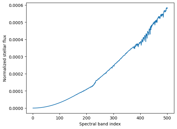
Check if the information about the normalized stellar flux per spectral band is read in correctly
[8]:
normalized_stellar_flux = read_normalized_stellar_flux(spectral_file)

plt.plot(
    normalized_stellar_flux.coord("spectral_band_index").points,
    normalized_stellar_flux.data,
)
plt.xlabel("Spectral band index")
plt.ylabel("Normalized stellar flux");
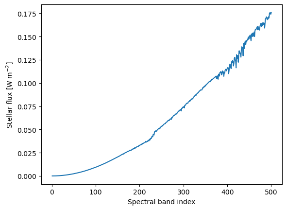
Calculate the stellar flux per spectral band
[9]:
stellar_flux = calc_stellar_flux(spectral_file, stellar_constant_at_1_au)

plt.plot(stellar_flux.coord("spectral_band_index").points, stellar_flux.data)
plt.xlabel("Spectral band index")
plt.ylabel("Stellar flux [W $m^{-2}$]");
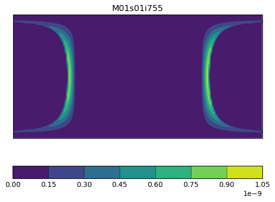
Check if you use the correct UM output by plotting the m01s01i755 field at a single spectral band
[10]:
qplt.contourf(planet_transmission_day[100, ...]);
Calculate transmission spectrum as a planet-to-star radius ratio
[11]:
rp_eff_over_rs = calc_transmission_spectrum(
    planet_transmission_day,
    spectral_file,
    stellar_constant_at_1_au,
    stellar_radius,
    planet_top_of_atmosphere,
    model=um,
)
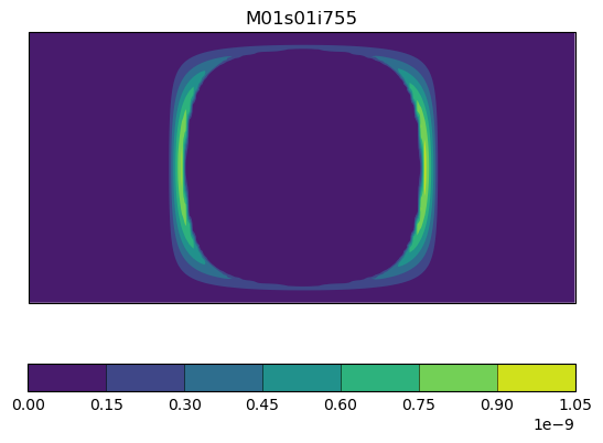
Calculate transmission spectrum averaged over the dayside and the nightside
[12]:
planet_transmission_night = iris.load_cube(TEST_DIR / "netcdf" / "planet_transmission_night.nc")
[13]:
qplt.contourf(planet_transmission_night[100, ...]);
[14]:
rp_eff_over_rs_night = calc_transmission_spectrum(
    planet_transmission_night,
    spectral_file,
    stellar_constant_at_1_au,
    stellar_radius,
    planet_top_of_atmosphere,
    model=um,
)
[15]:
rp_eff_over_rs_dn = calc_transmission_spectrum_day_night_average(
    planet_transmission_day,
    planet_transmission_night,
    add_shift=-1,
    spectral_file=spectral_file,
    stellar_constant_at_1_au=stellar_constant_at_1_au,
    stellar_radius=stellar_radius,
    planet_top_of_atmosphere=planet_top_of_atmosphere,
    model=um,
)
[16]:
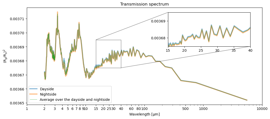
fig, ax = plt.subplots(figsize=(12, 5))
axins = ax.inset_axes([0.6, 0.6, 0.35, 0.35])
axins.set_xlim(15, 40)
axins.set_ylim(0.003675, 0.003695)
for _ax in (ax, axins):
    _ax.plot(
        rp_eff_over_rs.coord("spectral_band_centres").points * 1e6,
        rp_eff_over_rs.data**2,
        label="Dayside",
        linewidth=3,
        alpha=0.5,
    )
    _ax.plot(
        rp_eff_over_rs_night.coord("spectral_band_centres").points * 1e6,
        rp_eff_over_rs_night.data**2,
        label="Nightside",
        linewidth=3,
        alpha=0.5,
    )
    _ax.plot(
        rp_eff_over_rs_dn.coord("spectral_band_centres").points * 1e6,
        rp_eff_over_rs_dn.data**2,
        label="Average over the dayside and nightside",
        linewidth=0.5,
    )

ax.set_title("Transmission spectrum")
ax.set_xlabel("Wavelength [$\mu$m]")
ax.set_ylabel("($R_p/R_s)^2$")
ax.set_xscale("log")

xticks = np.concatenate(
    [
        np.arange(1, 11, 1),
        np.arange(15, 35, 5),
        np.arange(40, 120, 20),
        np.arange(500, 1400, 500),
        np.arange(10000, 10001, 500),
    ]
)
ax.set_xticks(xticks)
ax.set_xticklabels(xticks)
ax.indicate_inset_zoom(axins, edgecolor="black")
ax.legend(loc="lower left");
Check what the band limits are
[17]:
rp_eff_over_rs_dn.coord("spectral_band_upper_limit").points[:10]
[17]:
array([0.01      , 0.001     , 0.0005    , 0.00033333, 0.00025   ,
       0.0002    , 0.00016667, 0.00014286, 0.000125  , 0.00011111],
      dtype=float32)
[18]:
rp_eff_over_rs_dn.coord("spectral_band_lower_limit").points[:10]
[18]:
array([1.0000000e-03, 5.0000002e-04, 3.3333333e-04, 2.5000001e-04,
       1.9999999e-04, 1.6666666e-04, 1.4285714e-04, 1.2500001e-04,
       1.1111111e-04, 9.9999997e-05], dtype=float32)